
Reinforcement Learning: From Value-Iteration to Q-Learning to Deep-Q-Networks (DQNs)
Published:
Talking about different Reinforcement Learning algorithms in increasing order of complexity and how they relate to each other.
Introduction
Here, I try to highlight the main details of different reinforcement learning algorithms starting from the very basics, and smoothly transitioning to more complex ones like Deep Q Learning.
Markov Decision Process (MDP)
In order to understand value-iteration and everything after that, one needs to understand markov decision process. It is simply a system in which there can exist multiple different states, and one can move from one state to another by taking actions. It is generally represented as such:
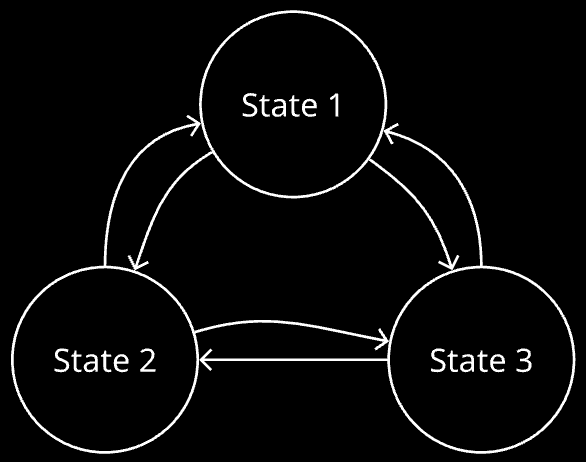
However, a more accurate/general representation is this, where it is not assumed that chosen an action from a state, the next state we will end up in is fixed:
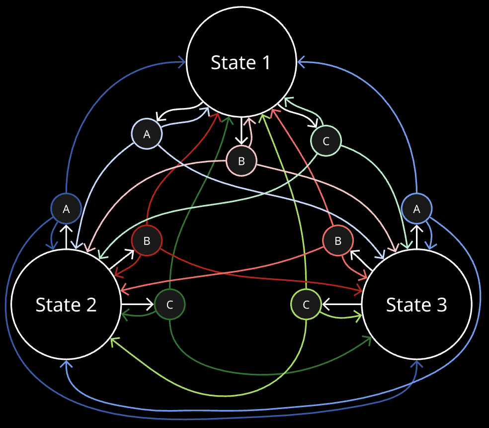
A, B, C here are actions which can possibly be taken from each state, and given current state s, and chosen action a, we may end up in any possible state with a certain probability. Set of probabilities driving this are called transition probabilities, which are intrinsic to the system.
More formally, intrinsic to the system, there is a set of transition probabilities. They denote that given a current state and chosen action from that state, what is the probability of landing in each of the states.
\[T:\mathcal{S}\times\mathcal{A}\times \mathcal{S}\to[0,1]\]where \(\mathcal{S}\) is the set of all possible states and \(\mathcal{A}\) is the set of all possible actions.
When we talk about learning a policy to take optimal decisions from each state in the system, it generally refers to something in the form of probabilities of choosing each possible action, given the current state.
\[\pi:\mathcal{S}\times\mathcal{A}\to[0,1]\]Return
In order to quantify goodness of policies, we associate with each decision (an action taken from a given current state), a reward value: if a good action was taken given the current circumstances, we get a reward, if not then maybe less reward.
\[r:\mathcal{S}\times\mathcal{A}\to\mathbb{R}\]A trajectory is defined as a sequence of states, actions and corresponding rewards (actions been taken from each state according to a policy), which takes us through many (possibly infinite) states in the system.
\[\tau=(s_{0},a_{0},r_{0},s_{1},a_{1},r_{1},s_{2},a_{2},r_{2},\cdots)\]Return of a trajectory is defined as the summation of all the rewards collected along the way.
\[R(\tau)=r_{0}+r_{1}+r_{2}+\cdots.\]I like to think of MDPs in the following form, with horizontal direction being time. This helps us to think about returns better, as a trajectory is a path in the graph from left to right.
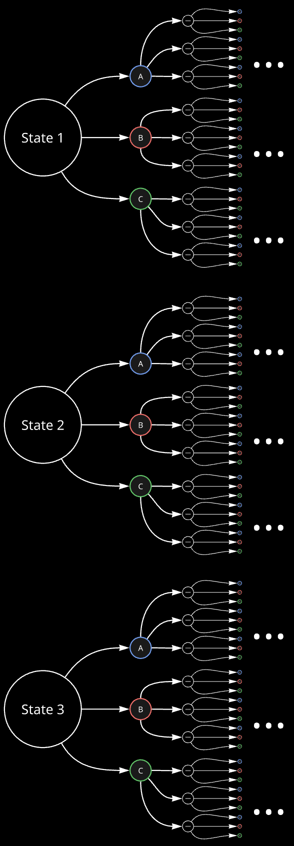
Here, the first column of circles corresponds to state at time 0 (\(s_0\)), second column (with blue, red, green circles) corresponds to action at time 0 (\(a_0\)), and so on…
Now, for a given starting state and policy, if we run the experiment of going through the states while choosing actions from a given policy many times, we get a return value each time, and if we average all of them, we get an expected return. However, if the trajectories are infinite in length each (meaning there is no possible way of ending the process by reaching a ‘final’ state), the expected value would be \(\infty\). It would be nice to be able to get a non-\(\infty\) number for the given starting state and policy, so that we can compare different policies on how they perform on average. Hence, we can introduce a discount factor: we multiply a number, \(\gamma^t\) to each reward, where \(t\) is the timepoint for which that reward is. \(\gamma\) is between 0 and 1 here, so that the sum converges. Hence, the discounted return for a single trajectory becomes:
\[R(\tau)=r_{0}+\gamma r_{1}+\gamma^{2}r_{2}+\cdots=\sum_{t=0}^{\infty}\gamma^{t}r_{t}\]And the expected return for a given starting state and a given policy can be represented as \(E_{a_{t}\sim\pi(s_{t})}\Big[R(\tau)\Big]\).
Value function
As defined just above, the expected return for a given starting state and policy can be a good measure by which we can compare different policies. This only is what we call the value function for a given policy, which takes as input the starting state, and gives the expected return:
\[V^{\pi}(s_{0})=E_{a_{t}\sim\pi(s_{t})}\Big[R(\tau)\Big]=E_{a_{t}\sim\pi(s_{t})}\Big[\sum_{t=0}^{\infty}\gamma^{t}r(s_{t},a_{t})\Big]\]So according to MDP visualization as discussed above, value function can be imagined as something like this:
Action-value function
Action-value function is defined for a starting state and action chosen from that state. It also gives the expected return, but for the given starting state-action combination.
\[Q^{\pi}(s_{0}, a_{0})= r(s_{0},a_{0}) + E_{a_{t}\sim\pi(s_{t}) ; t \ne0}\Big[R(\tau)\Big]=r(s_{0},a_{0}) + E_{a_{t}\sim\pi(s_{t}) ; t \ne0}\Big[\sum_{t=1}^{\infty}\gamma^{t}r(s_{t},a_{t})\Big]\]where \(\tau\) represents the set of trajectories with \(s_0\) and \(a_0\) at start.
It can be visualized as follows, for state-action combination as state 1 and action A:
Value-Iteration
Now that we have an idea of value function of a state and action-value function of a state-action pair, understanding value iteration is quite simple. Firstly, the value function of a state in terms of value functions of other states is this (the visualization shown above helps in appreciating it):
\[V^{\pi}(s)=\sum_{a\in\mathcal{A}}\pi(a\mid s)\Big[r(s,a)+\gamma\sum_{s^{\prime}\in\mathcal{S}}P(s^{\prime}\mid s,a)V^{\pi}(s^{\prime})\Big]\]The main point is this: If we initialize the value functions for all states with 0, and update all of them with respect to each other’s values, then as we do many iterations of such an update, the value functions of all states approaches their optimal value. Refer to Value Iteration, CS 188, UC Berkeley for more details. Hence, we can do exactly that, and obtain the value functions for all the states. Note that once we have that, we also know what action to take from each state for best expected return, because that depends on the value functions of other states only:
\[Q^{\pi}(s,a)=r(s,a)+\gamma\sum_{s^{\prime}\in\mathcal{S}}P(s^{\prime}\mid s,a)V^{\pi}(s^{\prime})\]We can either choose the best action each time or choose the actions probabilistically according to their expected return. Our policy function will accordingly be either deterministic (chooses always one action, given current state) or non-deterministic.
Q-Learning
When we don’t know the transition probabilities analytically in our system, we can gather an empirical estimate of that by updating action-value functions of state-action pairs, as we go through the system. More precisely, we initialize a policy, take actions according to it, and in each step we take, we use the value-function estimate thus far of the next state to improve the action-value function estimate of the just current state-action pair. Since the states that we will end up in, given an action from the current state would be reflective of the transition probabilities, the current action-value pair is updated with respect to possible next states in a weighted fashion, reflecting the real transition probabilities. Hence, here we are learning by doing.
So, suppose we were in state \(s_t\) and have just taken action \(a_t\) from it, and we end up in state \(s_{t+1}\). We can define a loss function as:
\[\ell = \Big[Q(s_t,a_t)-[r(s_t,a_t) + \gamma V(s_{t+1})]\Big]^2\]and update \(Q(s_t,a_t)\) using the following rule (\(\alpha\) is the learning rate):
\[Q(s_{t},a_{t})\leftarrow Q(s_{t},a_{t})-\alpha\nabla_{Q(s_{t},a_{t})}\ell\]This gives us the update equation:
\[Q(s_t,a_t) \leftarrow (1-\alpha)Q(s_{t},a_{t})+\alpha\Big(r({s_{t},a_{t}})+\gamma V(s_{t+1})\Big)\]If we assume that from a given state, we only choose the best policy in the fully trained state, then we can get an estimate of \(V(s_{t+1})\) as follows:
\[V(s_{t+1}) = \max_{a_{t+1} \in \mathcal{A}}(Q(s_{t+1}, a_{t+1}))\]Hence, using just estimates of just action-value functions for each state-action combination, we can iteratively explore the system, and gradually get closer to the actual values of them. The table storing the action-value functions for each state-action pair is generally called the q-table.
Deep-Q-Networks (single model)
For continuous systems, there would be infinite number of states. Hence, having something like a table, storing current estimates of action-value functions for all state-action pairs is not possible. For such cases, we make use of the fact that neural networks are universal function approximators. Optimally, the trained neural network can take in the continuous, decimal values identifying a state, and return the action-value function corresponding to each of the actions from that state. This is precisely what Deep-Q-Networks try to achieve.
Suppose in the system, each state is parameterized by 4 numbers, and there are 2 possible actions from each state. Possibly, we can have a neural network which will take the 4 numbers as input, and in last layer have 2 nodes, each corresponding to one of the possible actions. Hence, if its fully trained, we can plug in the value of the parameters of a state and get the action-value function for both the actions possible from the state. The update rule for such a network would be very similar to what we had for q-learning:
\[Q(s_t,a_t) \leftarrow (1-\alpha)Q(s_{t},a_{t})+\alpha\Big[r({s_{t},a_{t}})+\gamma \max_{a_{t+1} \in \mathcal{A}}\Big(Q(s_{t+1}, a_{t+1})\Big)\Big]\]Or we can simply formulate our loss function on which we can call .backward() and optimize our model’s parameters using any optimizer in pytorch. The loss function would be exactly what we discussed above:
According to our example, the value in the first node of last layer of the neural network would be \(Q(s_t,a_0)\) and the value in the second node of last layer of the neural network would be \(Q(s_t,a_1)\).
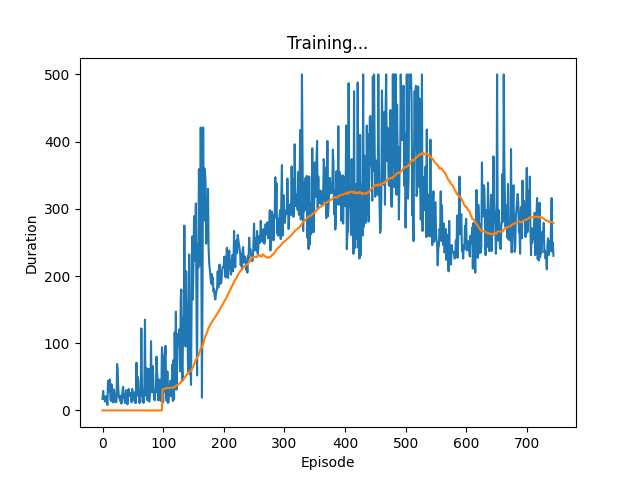
I tried an implementation of this on the cartpole task (inspired from this Pytorch tutorial), and the results looked like this:
Plotting the duration of each run looked like this (we would want the duration of runs to go high asap as that indicates the model knows how to keep the pole balanced for long by taking the correct decisions at each timepoint):
Deep-Q-Networks (double model)
It has been found that in many cases, having a separate, target neural network, which is attempted to be approached by the policy/online neural network, is helpful for faster and more stable training. This is exactly how the original implementation is, in the pytorch tutorial indicated above. The loss function for this setup becomes something like this:
\[\ell = \Big[Q(s_t,a_t)-\Big(r(s_t,a_t) + \gamma \max_{a_{t+1} \in \mathcal{A}}Q'(s_{t+1}, a_{t+1})\Big)\Big]^2\]where \(Q'(s_{t+1}, a_{t+1})\) is obtained using the target network, while \(Q(s_t,a_t)\) from the online network.
On trying this, the plot showing the duration of runs looks like this:
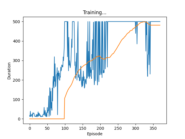
It is pretty convincing that learning is much faster (reaching max duration of 500 timepoints in around 250 iterations as opposed to around 500 in the case with single model), as well as more robust (the duration stays at 500 for many iterations, unlike the case for single model).
Conclusions
Talked about the different reinforcement learning algorithms starting from the very basics. This can be a useful resource when revisiting this topic and trying to remember nuances of it.
References
- https://inst.eecs.berkeley.edu/~cs188/textbook/mdp/value-iteration.html
- https://docs.pytorch.org/tutorials/intermediate/reinforcement_q_learning.html
- https://d2l.ai/