
Thinking about Backpropagation and Computation Graph in Pytorch
Published:
Guide to thinking about what happens when one calls tensor.backward() in pytorch.
Disclaimer: This is just an aid to visualizing the tensors in memory and what happens when we call .backward(). It is not a fully accurate description of what is happening under the hood. Please refer to pytorch documentation for exact details.
So even though I have tried to understand at a basic level what happens when we call torch.tensor.backward(), I have to think about it again every now and then whenever I see backpropagation or gradient computation mentioned somewhere while learning about something. Hence, I am making this guide, originally for my personal reference later, but I hope others find it useful too!
Error/Loss computation in a neural network
It all starts with the fact that in neural networks, computation of the error or loss is central for any learning to happen. The parameters of a neural network (weights and bias values, which are stored as tensors) go through many computations and finally, they yield a single value, the Error. To perform backpropagation then, we need the derivative of this Error value wrt every parameter (weight, bias etc.) of the neural network, so that we get an idea that how the error changes with a change in a certain parameter. This derivative value associated with each parameter is called its gradient in the context of neural networks. We would like to change the parameters in such a way that the error gets lesser.
In Pytorch, when we call .backward() function on a tensor, for all the tensors which were used to get the tensor on which .backward() was called, this gradient value gets computed. How just calling a single function on a single tensor leads to this (specifically from the angle of memory), is explained below.
Making some tensors, performing computations on them and getting a computational graph
Suppose we have a set of tensors, derived from each other:
tensor1 = torch.tensor([3], dtype = torch.float, requires_grad=True)
tensor2 = torch.tensor([4], dtype = torch.float, requires_grad=True)
# tensor([3.], requires_grad=True)
# tensor([4.], requires_grad=True)

tensor3 = tensor1 + tensor2
# tensor([7.], grad_fn=<AddBackward0>)

tensor4 = tensor3 * 2
# tensor([14.], grad_fn=<MulBackward0>)
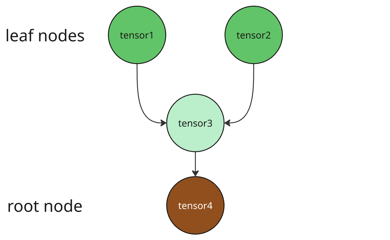
The computation graph for these would look like the following (I like to think of it as an upside down tree, because the independent/starting nodes (tensor1 and tensor2 in our case) are called the leaf nodes, but in the sequence of operations they come first, so an upside down tree fits the definition).
As we can see in the outputs, the tensors hold the information about which operation was (last) performed to obtain them. The tensor “holds” the information about what is the derivative of itself wrt its derivers \(\frac{dt}{dx}\).
Here is how our computation graph would roughly look like:
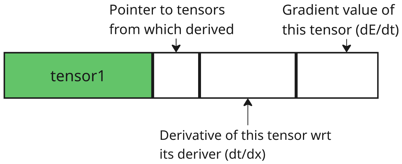
How to imagine a tensor in memory
I like to imagine a tensor in the memory as follows:
Which means that our expanded computation graph would look like the following:
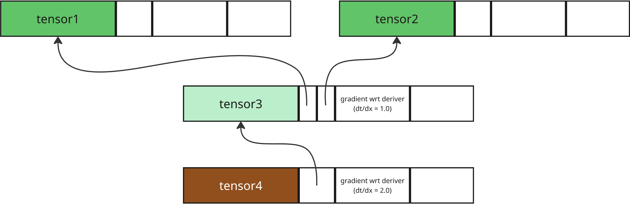
Calling tensor4.backward()
Hence, when we call tensor4.backward(), roughly, the following steps happen to get the gradient of each tensor (derivative of the final (root) tensor wrt it):

The gradient of the root tensor is simply 1 because its derivative with itself is 1.
The derivative of root wrt its deriver is multiplied by the gradient value of root (1.0), to get the gradient value of root’s deriver (2.0). Mathematically, \(\frac{dE}{dx}=\frac{dE}{dt}\frac{dt}{dx}\), where \(x\) denotes deriver of a tensor, \(t\) denotes current tensor (here root tensor), and \(E\) denotes the Error.
This process is repeated till we reach a leaf node, which doesn’t have deriver, and hence, we have the gradient value (again, keep in mind that this is derivative of root wrt any tensor) of each tensor.
References
- Visualizations made using miro tool: https://miro.com.
- I learnt about computation graphs in pytorch from here first. I would recommend this to any new learner: Introduction to PyTorch, UvA